Built-in Fitting Models in the models module

Lmfit provides several builtin fitting models in the models module. These pre-defined models each subclass from the model.Model class of the previous chapter and wrap relatively well-known functional forms, such as Gaussians, Lorentzian, and Exponentials that are used in a wide range of scientific domains. In fact, all the models are all based on simple, plain python functions defined in the lineshapes module. In addition to wrapping a function into a model.Model, these models also provide a guess() method that is intended to give a reasonable set of starting values from a data array that closely approximates the data to be fit.

As shown in the previous chapter, a key feature of the mode.Model class is that models can easily be combined to give a composite model.Model. Thus while some of the models listed here may seem pretty trivial (notably, ConstantModel and LinearModel), the main point of having these is to be able to used in composite models. For example, a Lorentzian plus a linear background might be represented as:

>>> from lmfit.models import LinearModel, LorentzianModel
>>> peak = LorentzianModel()
>>> background  = LinearModel()
>>> model = peak + background

All the models listed below are one dimensional, with an independent variable named x. Many of these models represent a function with a distinct peak, and so share common features. To maintain uniformity, common parameter names are used whenever possible. Thus, most models have a parameter called amplitude that represents the overall height (or area of) a peak or function, a center parameter that represents a peak centroid position, and a sigma parameter that gives a characteristic width. Some peak shapes also have a parameter fwhm, typically constrained by sigma to give the full width at half maximum.

After a list of builtin models, a few examples of their use is given.

Peak-like models

There are many peak-like models available. These include GaussianModel, LorentzianModel, VoigtModel and some less commonly used variations. The guess() methods for all of these make a fairly crude guess for the value of amplitude, but also set a lower bound of 0 on the value of sigma.

GaussianModel

class GaussianModel(missing=None[, prefix=''[, name=None[, **kws]]])

A model based on a Gaussian or normal distribution lineshape. Parameter names: amplitude, center, and sigma. In addition, a constrained parameter fwhm is included.

\[f(x; A, \mu, \sigma) = \frac{A}{\sigma\sqrt{2\pi}} e^{[{-{(x-\mu)^2}/{{2\sigma}^2}}]}\]

where the parameter amplitude corresponds to \(A\), center to \(\mu\), and sigma to \(\sigma\). The Full-Width at Half-Maximum is \(2\sigma\sqrt{2\ln{2}}\), approximately \(2.3548\sigma\)

LorentzianModel

class LorentzianModel(missing=None[, prefix=''[, name=None[, **kws]]])

A model based on a Lorentzian or Cauchy-Lorentz distribution function. Parameter names: amplitude, center, and sigma. In addition, a constrained parameter fwhm is included.

\[f(x; A, \mu, \sigma) = \frac{A}{\pi} \big[\frac{\sigma}{(x - \mu)^2 + \sigma^2}\big]\]

where the parameter amplitude corresponds to \(A\), center to \(\mu\), and sigma to \(\sigma\). The Full-Width at Half-Maximum is \(2\sigma\).

VoigtModel

class VoigtModel(missing=None[, prefix=''[, name=None[, **kws]]])

A model based on a Voigt distribution function. Parameter names: amplitude, center, and sigma. A gamma parameter is also available. By default, it is constrained to have value equal to sigma, though this can be varied independently. In addition, a constrained parameter fwhm is included. The definition for the Voigt function used here is

\[f(x; A, \mu, \sigma, \gamma) = \frac{A \textrm{Re}[w(z)]}{\sigma\sqrt{2 \pi}}\]

where

\[\begin{eqnarray*} z &=& \frac{x-\mu +i\gamma}{\sigma\sqrt{2}} \\ w(z) &=& e^{-z^2}{\operatorname{erfc}}(-iz) \end{eqnarray*}\]

and erfc() is the complimentary error function. As above, amplitude corresponds to \(A\), center to \(\mu\), and sigma to \(\sigma\). The parameter gamma corresponds to \(\gamma\). If gamma is kept at the default value (constrained to sigma), the full width at half maximum is approximately \(3.6013\sigma\).

PseudoVoigtModel

class PseudoVoigtModel(missing=None[, prefix=''[, name=None[, **kws]]])

a model based on a pseudo-Voigt distribution function, which is a weighted sum of a Gaussian and Lorentzian distribution functions with the same values for amplitude (\(A\)), center (\(\mu\)) and sigma (\(\sigma\)), and a parameter fraction (\(\alpha\)) in

\[f(x; A, \mu, \sigma, \alpha) = (1-\alpha)\frac{A}{\pi} \big[\frac{\sigma}{(x - \mu)^2 + \sigma^2}\big] + \frac{\alpha A}{\pi} \big[\frac{\sigma}{(x - \mu)^2 + \sigma^2}\big]\]

The guess() function always gives a starting value for fraction of 0.5

Pearson7Model

class Pearson7Model(missing=None[, prefix=''[, name=None[, **kws]]])

A model based on a Pearson VII distribution. This is a Lorenztian-like distribution function. It has the usual parameters amplitude (\(A\)), center (\(\mu\)) and sigma (\(\sigma\)), and also an exponent (\(m\)) in

\[f(x; A, \mu, \sigma, m) = \frac{A}{\sigma{\beta(m-\frac{1}{2}, \frac{1}{2})}} \bigl[1 + \frac{(x-\mu)^2}{\sigma^2} \bigr]^{-m}\]

where \(\beta\) is the beta function (see scipy.special.beta() in scipy.special). The guess() function always gives a starting value for exponent of 1.5.

StudentsTModel

class StudentsTModel(missing=None[, prefix=''[, name=None[, **kws]]])

A model based on a Student’s t distribution function, with the usual parameters amplitude (\(A\)), center (\(\mu\)) and sigma (\(\sigma\)) in

\[f(x; A, \mu, \sigma) = \frac{A \Gamma(\frac{\sigma+1}{2})} {\sqrt{\sigma\pi}\,\Gamma(\frac{\sigma}{2})} \Bigl[1+\frac{(x-\mu)^2}{\sigma}\Bigr]^{-\frac{\sigma+1}{2}}\]

where \(\Gamma(x)\) is the gamma function.

BreitWignerModel

class BreitWignerModel(missing=None[, prefix=''[, name=None[, **kws]]])

A model based on a Breit-Wigner-Fano function. It has the usual parameters amplitude (\(A\)), center (\(\mu\)) and sigma (\(\sigma\)), plus q (\(q\)) in

\[f(x; A, \mu, \sigma, q) = \frac{A (q\sigma/2 + x - \mu)^2}{(\sigma/2)^2 + (x - \mu)^2}\]

LognormalModel

class LognormalModel(missing=None[, prefix=''[, name=None[, **kws]]])

A model based on the Log-normal distribution function. It has the usual parameters amplitude (\(A\)), center (\(\mu\)) and sigma (\(\sigma\)) in

\[f(x; A, \mu, \sigma) = \frac{A e^{-(\ln(x) - \mu)/ 2\sigma^2}}{x}\]

DampedOcsillatorModel

class DampedOcsillatorModel(missing=None[, prefix=''[, name=None[, **kws]]])

A model based on the Damped Harmonic Oscillator Amplitude. It has the usual parameters amplitude (\(A\)), center (\(\mu\)) and sigma (\(\sigma\)) in

\[f(x; A, \mu, \sigma) = \frac{A}{\sqrt{ [1 - (x/\mu)^2]^2 + (2\sigma x/\mu)^2}}\]

ExponentialGaussianModel

class ExponentialGaussianModel(missing=None[, prefix=''[, name=None[, **kws]]])

A model of an Exponentially modified Gaussian distribution. It has the usual parameters amplitude (\(A\)), center (\(\mu\)) and sigma (\(\sigma\)), and also gamma (\(\gamma\)) in

\[f(x; A, \mu, \sigma, \gamma) = \frac{A\gamma}{2} \exp\bigl[\gamma({\mu - x + \gamma\sigma^2/2})\bigr] {\operatorname{erfc}}\Bigl(\frac{\mu + \gamma\sigma^2 - x}{\sqrt{2}\sigma}\Bigr)\]

where erfc() is the complimentary error function.

SkewedGaussianModel

class SkewedGaussianModel(missing=None[, prefix=''[, name=None[, **kws]]])

A variation of the above model, this is a Skewed normal distribution. It has the usual parameters amplitude (\(A\)), center (\(\mu\)) and sigma (\(\sigma\)), and also gamma (\(\gamma\)) in

\[ f(x; A, \mu, \sigma, \gamma) = \frac{A}{\sigma\sqrt{2\pi}} e^{[{-{(x-\mu)^2}/{{2\sigma}^2}}]} \Bigl\{ 1 + {\operatorname{erf}}\bigl[ \frac{\gamma(x-\mu)}{\sigma\sqrt{2\pi}} \bigr] \Bigr\}\]

where erf() is the error function.

DonaichModel

class DonaichModel(missing=None[, prefix=''[, name=None[, **kws]]])

A model of an Doniach Sunjic asymmetric lineshape, used in photo-emission. With the usual parameters amplitude (\(A\)), center (\(\mu\)) and sigma (\(\sigma\)), and also gamma (\(\gamma\)) in

\[f(x; A, \mu, \sigma, \gamma) = A\frac{\cos\bigl[\pi\gamma/2 + (1-\gamma) \arctan{(x - \mu)}/\sigma\bigr]} {\bigr[1 + (x-\mu)/\sigma\bigl]^{(1-\gamma)/2}}\]

Linear and Polynomial Models

These models correspond to polynomials of some degree. Of course, lmfit is a very inefficient way to do linear regression (see numpy.polyfit() or scipy.stats.linregress()), but these models may be useful as one of many components of composite model.

ConstantModel

class ConstantModel(missing=None[, prefix=''[, name=None[, **kws]]])

a class that consists of a single value, c. This is constant in the sense of having no dependence on the independent variable x, not in the sense of being non-varying. To be clear, c will be a variable Parameter.

LinearModel

class LinearModel(missing=None[, prefix=''[, name=None[, **kws]]])

a class that gives a linear model:

\[f(x; m, b) = m x + b\]

with parameters slope for \(m\) and intercept for \(b\).

QuadraticModel

class QuadraticModel(missing=None[, prefix=''[, name=None[, **kws]]])

a class that gives a quadratic model:

\[f(x; a, b, c) = a x^2 + b x + c\]

with parameters a, b, and c.

ParabolicModel

class ParabolicModel(missing=None[, prefix=''[, name=None[, **kws]]])

same as QuadraticModel.

PolynomialModel

class PolynomialModel(degree, missing=None[, prefix=''[, name=None[, **kws]]])

a class that gives a polynomial model up to degree (with maximum value of 7).

\[f(x; c_0, c_1, \ldots, c_7) = \sum_{i=0, 7} c_i x^i\]

with parameters c0, c1, ..., c7. The supplied degree will specify how many of these are actual variable parameters. This uses numpy.polyval() for its calculation of the polynomial.

Step-like models

Two models represent step-like functions, and share many characteristics.

StepModel

class StepModel(form='linear'[, missing=None[, prefix=''[, name=None[, **kws]]]])

A model based on a Step function, with four choices for functional form. The step function starts with a value 0, and ends with a value of \(A\) (amplitude), rising to \(A/2\) at \(\mu\) (center), with \(\sigma\) (sigma) setting the characteristic width. The supported functional forms are linear (the default), atan or arctan for an arc-tangent function, erf for an error function, or logistic for a logistic function. The forms are

\[\begin{eqnarray*} & f(x; A, \mu, \sigma, {\mathrm{form={}'linear{}'}}) & = A \min{[1, \max{(0, \alpha)}]} \\ & f(x; A, \mu, \sigma, {\mathrm{form={}'arctan{}'}}) & = A [1/2 + \arctan{(\alpha)}/{\pi}] \\ & f(x; A, \mu, \sigma, {\mathrm{form={}'erf{}'}}) & = A [1 + {\operatorname{erf}}(\alpha)]/2 \\ & f(x; A, \mu, \sigma, {\mathrm{form={}'logistic{}'}})& = A [1 - \frac{1}{1 + e^{\alpha}} ] \end{eqnarray*}\]

where \(\alpha = (x - \mu)/{\sigma}\).

RectangleModel

class RectangleModel(form='linear'[, missing=None[, prefix=''[, name=None[, **kws]]]])

A model based on a Step-up and Step-down function of the same form. The same choices for functional form as for StepModel are supported, with linear as the default. The function starts with a value 0, and ends with a value of \(A\) (amplitude), rising to \(A/2\) at \(\mu_1\) (center1), with \(\sigma_1\) (sigma1) setting the characteristic width. It drops to rising to \(A/2\) at \(\mu_2\) (center2), with characteristic width \(\sigma_2\) (sigma2).

\[\begin{eqnarray*} &f(x; A, \mu, \sigma, {\mathrm{form={}'linear{}'}}) &= A \{ \min{[1, \max{(0, \alpha_1)}]} + \min{[-1, \max{(0, \alpha_2)}]} \} \\ &f(x; A, \mu, \sigma, {\mathrm{form={}'arctan{}'}}) &= A [\arctan{(\alpha_1)} + \arctan{(\alpha_2)}]/{\pi} \\ &f(x; A, \mu, \sigma, {\mathrm{form={}'erf{}'}}) &= A [{\operatorname{erf}}(\alpha_1) + {\operatorname{erf}}(\alpha_2)]/2 \\ &f(x; A, \mu, \sigma, {\mathrm{form={}'logistic{}'}}) &= A [1 - \frac{1}{1 + e^{\alpha_1}} - \frac{1}{1 + e^{\alpha_2}} ] \end{eqnarray*}\]

where \(\alpha_1 = (x - \mu_1)/{\sigma_1}\) and \(\alpha_2 = -(x - \mu_2)/{\sigma_2}\).

Exponential and Power law models

ExponentialModel

class ExponentialModel(missing=None[, prefix=''[, name=None[, **kws]]])

A model based on an exponential decay function. With parameters named amplitude (\(A\)), and decay (\(\tau\)), this has the form:

\[f(x; A, \tau) = A e^{-x/\tau}\]

PowerLawModel

class PowerLawModel(missing=None[, prefix=''[, name=None[, **kws]]])

A model based on a Power Law. With parameters named amplitude (\(A\)), and exponent (\(k\)), this has the form:

\[f(x; A, k) = A x^k\]

User-defined Models

As shown in the previous chapter (Modeling Data and Curve Fitting), it is fairly straightforward to build fitting models from parametrized python functions. The number of model classes listed so far in the present chapter should make it clear that this process is not too difficult. Still, it is sometimes desirable to build models from a user-supplied function. This may be especially true if model-building is built-in to some larger library or application for fitting in which the user may not be able to easily build and use a new model from python code.

The ExpressionModel allows a model to be built from a user-supplied expression. This uses the asteval module also used for mathematical constraints as discussed in Using Mathematical Constraints.

ExpressionModel

class ExpressionModel(expr, independent_vars=None, init_script=None, missing=None, prefix='', name=None, **kws)

A model using the user-supplied mathematical expression, which can be nearly any valid Python expresion.

Parameters:

• expr (string) – expression use to build model
• init_script (None (default) or string) – python script to run before parsing and evaluating expression.
• independent_vars (None (default) or list of strings for independent variables.) – list of argument names to func that are independent variables.

with other parameters passed to model.Model.

Since the point of this model is that an arbitrary expression will be supplied, the determination of what are the parameter names for the model happens when the model is created. To do this, the expression is parsed, and all symbol names are found. Names that are already known (there are over 500 function and value names in the asteval namespace, including most python builtins, more than 200 functions inherited from numpy, and more than 20 common lineshapes defined in the lineshapes module) are not converted to parameters. Unrecognized name are expected to be names either of parameters or independent variables. If independent_vars is the default value of None, and if the expression contains a variable named x, that will be used as the independent variable. Otherwise, independent_vars must be given.

For example, if one creates an ExpressionModel as:

>>> mod = ExpressionModel('off + amp * exp(-x/x0) * sin(x*phase)')

The name exp will be recognized as the exponent function, so the model will be interpreted to have parameters named off, amp, x0 and phase, and x will be assumed to be the sole independent variable. In general, there is no obvious way to set default parameter values or parameter hints for bounds, so this will have to be handled explicitly.

To evaluate this model, you might do the following:

>>> x = numpy.linspace(0, 10, 501)
>>> params = mod.make_params(off=0.25, amp=1.0, x0=2.0, phase=0.04)
>>> y = mod.eval(params, x=x)

While many custom models can be built with a single line expression (especially since the names of the lineshapes like gaussian, lorentzian and so on, as well as many numpy functions, are available), more complex models will inevitably require multiple line functions. You can include such Python code with the init_script argument. The text of this script is evaluated when the model is initialized (and before the actual expression is parsed), so that you can define functions to be used in your expression.

As a probably unphysical example, to make a model that is the derivative of a Gaussian function times the logarithm of a Lorentzian function you may could to define this in a script:

>>> script = """
def mycurve(x, amp, cen, sig):
    loren = lorentzian(x, amplitude=amp, center=cen, sigma=sig)
    gauss = gaussian(x, amplitude=amp, center=cen, sigma=sig)
    return log(loren)*gradient(gauss)/gradient(x)
"""

and then use this with ExpressionModel as:

>>> mod = ExpressionModel('mycurve(x, height, mid, wid)',
                          init_script=script,
                          independent_vars=['x'])

As above, this will interpret the parameter names to be height, mid, and wid, and build a model that can be used to fit data.

Example 1: Fit Peaked data to Gaussian, Lorentzian, and Voigt profiles

Here, we will fit data to three similar line shapes, in order to decide which might be the better model. We will start with a Gaussian profile, as in the previous chapter, but use the built-in GaussianModel instead of one we write ourselves. This is a slightly different version from the one in previous example in that the parameter names are different, and have built-in default values. So, we’ll simply use:

from numpy import loadtxt
from lmfit.models import GaussianModel

data = loadtxt('test_peak.dat')
x = data[:, 0]
y = data[:, 1]

mod = GaussianModel()
pars = mod.guess(y, x=x)
out  = mod.fit(y, pars, x=x)
print(out.fit_report(min_correl=0.25))

which prints out the results:

[[Model]]
    gaussian
[[Fit Statistics]]
    # function evals   = 21
    # data points      = 401
    # variables        = 3
    chi-square         = 29.994
    reduced chi-square = 0.075
[[Variables]]
    amplitude:   30.3135571 +/- 0.157126 (0.52%) (init= 29.08159)
    center:      9.24277049 +/- 0.007374 (0.08%) (init= 9.25)
    fwhm:        2.90156963 +/- 0.017366 (0.60%)  == '2.3548200*sigma'
    sigma:       1.23218319 +/- 0.007374 (0.60%) (init= 1.35)
[[Correlations]] (unreported correlations are <  0.250)
    C(amplitude, sigma)          =  0.577

[We see a few interesting differences from the results of the previous

chapter. First, the parameter names are longer. Second, there is a fwhm parameter, defined as \(\sim 2.355\sigma\). And third, the automated initial guesses are pretty good. A plot of the fit shows not such a great fit:

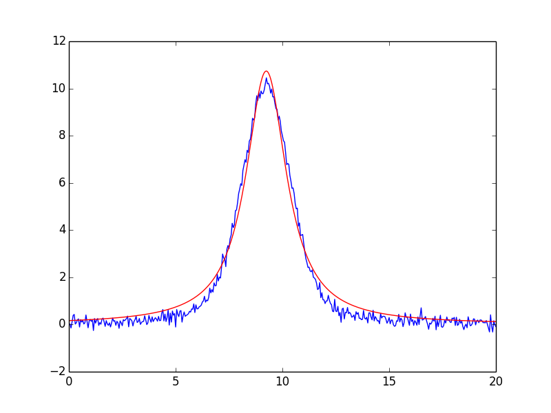
Fit to peak with Gaussian (left) and Lorentzian (right) models.

suggesting that a different peak shape, with longer tails, should be used. Perhaps a Lorentzian would be better? To do this, we simply replace GaussianModel with LorentzianModel to get a LorentzianModel:

from lmfit.models import LorentzianModel
mod = LorentzianModel()
pars = mod.guess(y, x=x)
out  = mod.fit(y, pars, x=x)
print(out.fit_report(min_correl=0.25))

Predictably, the first thing we try gives results that are worse:

[[Model]]
    lorentzian
[[Fit Statistics]]
    # function evals   = 25
    # data points      = 401
    # variables        = 3
    chi-square         = 53.754
    reduced chi-square = 0.135
[[Variables]]
    amplitude:   38.9728645 +/- 0.313857 (0.81%) (init= 36.35199)
    center:      9.24438944 +/- 0.009275 (0.10%) (init= 9.25)
    fwhm:        2.30969034 +/- 0.026312 (1.14%)  == '2.0000000*sigma'
    sigma:       1.15484517 +/- 0.013156 (1.14%) (init= 1.35)
[[Correlations]] (unreported correlations are <  0.250)
    C(amplitude, sigma)          =  0.709

with the plot shown on the right in the figure above.

A Voigt model does a better job. Using VoigtModel, this is as simple as:

from lmfit.models import VoigtModel
mod = VoigtModel()
pars = mod.guess(y, x=x)
out  = mod.fit(y, pars, x=x)
print(out.fit_report(min_correl=0.25))

which gives:

[[Model]]
    voigt
[[Fit Statistics]]
    # function evals   = 17
    # data points      = 401
    # variables        = 3
    chi-square         = 14.545
    reduced chi-square = 0.037
[[Variables]]
    amplitude:   35.7554017 +/- 0.138614 (0.39%) (init= 43.62238)
    center:      9.24411142 +/- 0.005054 (0.05%) (init= 9.25)
    fwhm:        2.62951718 +/- 0.013269 (0.50%)  == '3.6013100*sigma'
    gamma:       0.73015574 +/- 0.003684 (0.50%)  == 'sigma'
    sigma:       0.73015574 +/- 0.003684 (0.50%) (init= 0.8775)
[[Correlations]] (unreported correlations are <  0.250)
    C(amplitude, sigma)          =  0.651

with the much better value for \(\chi^2\) and the obviously better match to the data as seen in the figure below (left).

Fit to peak with Voigt model (left) and Voigt model with gamma varying independently of sigma (right).

The Voigt function has a \(\gamma\) parameter (gamma) that can be distinct from sigma. The default behavior used above constrains gamma to have exactly the same value as sigma. If we allow these to vary separately, does the fit improve? To do this, we have to change the gamma parameter from a constrained expression and give it a starting value:

mod = VoigtModel()
pars = mod.guess(y, x=x)
pars['gamma'].set(value=0.7, vary=True, expr='')

out  = mod.fit(y, pars, x=x)
print(out.fit_report(min_correl=0.25))

which gives:

[[Model]]
    voigt
[[Fit Statistics]]
    # function evals   = 21
    # data points      = 401
    # variables        = 4
    chi-square         = 10.930
    reduced chi-square = 0.028
[[Variables]]
    amplitude:   34.1914716 +/- 0.179468 (0.52%) (init= 43.62238)
    center:      9.24374845 +/- 0.004419 (0.05%) (init= 9.25)
    fwhm:        3.22385491 +/- 0.050974 (1.58%)  == '3.6013100*sigma'
    gamma:       0.52540157 +/- 0.018579 (3.54%) (init= 0.7)
    sigma:       0.89518950 +/- 0.014154 (1.58%) (init= 0.8775)
[[Correlations]] (unreported correlations are <  0.250)
    C(amplitude, gamma)          =  0.821

and the fit shown on the right above.

Comparing the two fits with the Voigt function, we see that \(\chi^2\) is definitely improved with a separately varying gamma parameter. In addition, the two values for gamma and sigma differ significantly – well outside the estimated uncertainties. Even more compelling, reduced \(\chi^2\) is improved even though a fourth variable has been added to the fit. In the simplest statistical sense, this suggests that gamma is a significant variable in the model.

This example shows how easy it can be to alter and compare fitting models for simple problems. The example is included in the doc_peakmodels.py file in the examples directory.

Example 2: Fit data to a Composite Model with pre-defined models

Here, we repeat the point made at the end of the last chapter that instances of model.Model class can be added them together to make a composite model. But using the large number of built-in models available, this is very simple. An example of a simple fit to a noisy step function plus a constant:

#!/usr/bin/env python
#<examples/doc_stepmodel.py>
import numpy as np
from lmfit.models import StepModel, LinearModel

import matplotlib.pyplot as plt

x = np.linspace(0, 10, 201)
y = np.ones_like(x)
y[:48] = 0.0
y[48:77] = np.arange(77-48)/(77.0-48)
y = 110.2 * (y + 9e-3*np.random.randn(len(x))) + 12.0 + 2.22*x

step_mod = StepModel(form='erf', prefix='step_')
line_mod = LinearModel(prefix='line_')

pars =  line_mod.make_params(intercept=y.min(), slope=0)
pars += step_mod.guess(y, x=x, center=2.5)

mod = step_mod + line_mod
out = mod.fit(y, pars, x=x)

print(out.fit_report())

plt.plot(x, y)
plt.plot(x, out.init_fit, 'k--')
plt.plot(x, out.best_fit, 'r-')
plt.show()
#<end examples/doc_stepmodel.py>

After constructing step-like data, we first create a StepModel telling it to use the erf form (see details above), and a ConstantModel. We set initial values, in one case using the data and guess() method for the initial step function paramaters, and make_params() arguments for the linear component. After making a composite model, we run fit() and report the results, which give:

[[Model]]
 Composite Model:
    step(prefix='step_',form='erf')
    linear(prefix='line_')
[[Fit Statistics]]
    # function evals   = 49
    # data points      = 201
    # variables        = 5
    chi-square         = 633.465
    reduced chi-square = 3.232
[[Variables]]
    line_intercept:   11.5685248 +/- 0.285611 (2.47%) (init= 10.72406)
    line_slope:       2.03270159 +/- 0.096041 (4.72%) (init= 0)
    step_amplitude:   112.270535 +/- 0.674790 (0.60%) (init= 136.3006)
    step_center:      3.12343845 +/- 0.005370 (0.17%) (init= 2.5)
    step_sigma:       0.67468813 +/- 0.011336 (1.68%) (init= 1.428571)
[[Correlations]] (unreported correlations are <  0.100)
    C(step_amplitude, step_sigma)  =  0.564
    C(line_intercept, step_center)  =  0.428
    C(step_amplitude, step_center)  =  0.109

with a plot of

Example 3: Fitting Multiple Peaks – and using Prefixes

As shown above, many of the models have similar parameter names. For composite models, this could lead to a problem of having parameters for different parts of the model having the same name. To overcome this, each model.Model can have a prefix attribute (normally set to a blank string) that will be put at the beginning of each parameter name. To illustrate, we fit one of the classic datasets from the NIST StRD suite involving a decaying exponential and two gaussians.

#!/usr/bin/env python
#<examples/doc_nistgauss.py>
import numpy as np
from lmfit.models import GaussianModel, ExponentialModel
import sys
import matplotlib.pyplot as plt

dat = np.loadtxt('NIST_Gauss2.dat')
x = dat[:, 1]
y = dat[:, 0]

exp_mod = ExponentialModel(prefix='exp_')
pars = exp_mod.guess(y, x=x)

gauss1  = GaussianModel(prefix='g1_')
pars.update( gauss1.make_params())

pars['g1_center'].set(105, min=75, max=125)
pars['g1_sigma'].set(15, min=3)
pars['g1_amplitude'].set(2000, min=10)

gauss2  = GaussianModel(prefix='g2_')

pars.update(gauss2.make_params())

pars['g2_center'].set(155, min=125, max=175)
pars['g2_sigma'].set(15, min=3)
pars['g2_amplitude'].set(2000, min=10)

mod = gauss1 + gauss2 + exp_mod


init = mod.eval(pars, x=x)
plt.plot(x, y)
plt.plot(x, init, 'k--')

out = mod.fit(y, pars, x=x)

print(out.fit_report(min_correl=0.5))

plt.plot(x, out.best_fit, 'r-')
plt.show()
#<end examples/doc_nistgauss.py>

where we give a separate prefix to each model (they all have an amplitude parameter). The prefix values are attached transparently to the models.

MN—-: Note that the calls to make_param() used the bare name, without the prefix. We could have used them, but because we used the individual model gauss1 and gauss2, there was no need.

Note also in the example here that we explicitly set bounds on many of the parameter values.

The fit results printed out are:

[[Model]]
 Composite Model:
    gaussian(prefix='g1_')
    gaussian(prefix='g2_')
    exponential(prefix='exp_')
[[Fit Statistics]]
    # function evals   = 55
    # data points      = 250
    # variables        = 8
    chi-square         = 1247.528
    reduced chi-square = 5.155
[[Variables]]
    exp_amplitude:   99.0183291 +/- 0.537487 (0.54%) (init= 162.2102)
    exp_decay:       90.9508788 +/- 1.103104 (1.21%) (init= 93.24905)
    g1_amplitude:    4257.77384 +/- 42.38354 (1.00%) (init= 2000)
    g1_center:       107.030955 +/- 0.150068 (0.14%) (init= 105)
    g1_fwhm:         39.2609205 +/- 0.377907 (0.96%)  == '2.3548200*g1_sigma'
    g1_sigma:        16.6725781 +/- 0.160482 (0.96%) (init= 15)
    g2_amplitude:    2493.41747 +/- 36.16907 (1.45%) (init= 2000)
    g2_center:       153.270103 +/- 0.194665 (0.13%) (init= 155)
    g2_fwhm:         32.5128760 +/- 0.439860 (1.35%)  == '2.3548200*g2_sigma'
    g2_sigma:        13.8069474 +/- 0.186791 (1.35%) (init= 15)
[[Correlations]] (unreported correlations are <  0.500)
    C(g1_amplitude, g1_sigma)    =  0.824
    C(g2_amplitude, g2_sigma)    =  0.815
    C(g1_sigma, g2_center)       =  0.684
    C(g1_amplitude, g2_center)   =  0.648
    C(g1_center, g2_center)      =  0.621
    C(g1_center, g1_sigma)       =  0.507

We get a very good fit to this challenging problem (described at the NIST site as of average difficulty, but the tests there are generally hard) by applying reasonable initial guesses and putting modest but explicit bounds on the parameter values. This fit is shown on the left:

One final point on setting initial values. From looking at the data itself, we can see the two Gaussian peaks are reasonably well separated but do overlap. Furthermore, we can tell that the initial guess for the decaying exponential component was poorly estimated because we used the full data range. We can simplify the initial parameter values by using this, and by defining an index_of() function to limit the data range. That is, with:

def index_of(arrval, value):
    "return index of array *at or below* value "
    if value < min(arrval):  return 0
    return max(np.where(arrval<=value)[0])

ix1 = index_of(x,  75)
ix2 = index_of(x, 135)
ix3 = index_of(x, 175)

exp_mod.guess(y[:ix1], x=x[:ix1])
gauss1.guess(y[ix1:ix2], x=x[ix1:ix2])
gauss2.guess(y[ix2:ix3], x=x[ix2:ix3])

we can get a better initial estimate, and the fit converges in fewer steps, getting to identical values (to the precision printed out in the report), and without any bounds on parameters at all:

[[Model]]
 Composite Model:
    gaussian(prefix='g1_')
    gaussian(prefix='g2_')
    exponential(prefix='exp_')
[[Fit Statistics]]
    # function evals   = 46
    # data points      = 250
    # variables        = 8
    chi-square         = 1247.528
    reduced chi-square = 5.155
[[Variables]]
    exp_amplitude:   99.0183281 +/- 0.537487 (0.54%) (init= 94.53724)
    exp_decay:       90.9508863 +/- 1.103105 (1.21%) (init= 111.1985)
    g1_amplitude:    4257.77321 +/- 42.38338 (1.00%) (init= 2126.432)
    g1_center:       107.030954 +/- 0.150067 (0.14%) (init= 106.5)
    g1_fwhm:         39.2609141 +/- 0.377905 (0.96%)  == '2.3548200*g1_sigma'
    g1_sigma:        16.6725754 +/- 0.160481 (0.96%) (init= 14.5)
    g2_amplitude:    2493.41766 +/- 36.16948 (1.45%) (init= 1878.892)
    g2_center:       153.270100 +/- 0.194667 (0.13%) (init= 150)
    g2_fwhm:         32.5128777 +/- 0.439866 (1.35%)  == '2.3548200*g2_sigma'
    g2_sigma:        13.8069481 +/- 0.186794 (1.35%) (init= 15)
[[Correlations]] (unreported correlations are <  0.500)
    C(g1_amplitude, g1_sigma)    =  0.824
    C(g2_amplitude, g2_sigma)    =  0.815
    C(g1_sigma, g2_center)       =  0.684
    C(g1_amplitude, g2_center)   =  0.648
    C(g1_center, g2_center)      =  0.621
    C(g1_center, g1_sigma)       =  0.507

This example is in the file doc_nistgauss2.py in the examples folder, and the fit result shown on the right above shows an improved initial estimate of the data.